
Learning Neural Networks the Practical Way— By Building Them in Python
There’s no getting around it. Neural networks are complicated. And hard to understand. It is hard to know where to start when using them. There are so many architectural decisions, hyperparameters, and other settings to consider, that, when building models, it can feel like mashing random values together until something works. That was my experience, at least, when I began my fascinating journey into learning neural networks.

So, I decided to start at the beginning. I started small, with arrays of weights, biases, and data records, and layered concepts standard in modern neural networks on top of each other. By the end, I had a fully working, generalized neural network framework built from scratch in python. Read on to see the highlights of the process.
This article is based on work I did in three jupyter notebooks. Check these notebooks out if you want to see the full implementations of these concepts:
Most of the information in those notebooks comes from two sources. Firstly, Stanford’s CS231n (Convolutional Neural Networks for Visual Recognition) provided a great view into the theoretical principles behind classification models first and neural networks second. Second, Neural Networks from Scratch in Python covers all practical steps for implementing these models in python, making it a great resource for practical learning.
This article is another entry in my series exploring the fundamentals of machine learning through example-based learning, and the first one that explores advanced neural network models. Click here to see other entries in this series.
Getting Started: A Sample Dataset and the Neural Network Architecture
Understanding Neural networks begins with understanding how classification models work. You can look at either of the two previous posts in this series to get an idea for how that works. But here is a quick rundown:
To start, you need a set of data that you wish to make predictions on. Let’s say, for example, we have a set of points laid out on a coordinate plane like this:
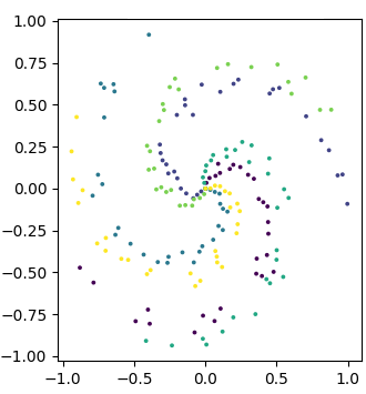
| x | y | class (color) |
| 0 | -0.85 | 1 (blue) |
| 0.75 | 0.25 | 2 (purple) |
| … | … | … |
This data consists of data points with an x coordinate, a y coordinate, and color. Let’s say, on this data, that we would like to predict what color a point will be using only the x and y coordinates. By looking at the graph, you can see that this should be possible. If a point is located at a certain location, by looking at it, you can usually tell which color group it should be a part of. We want to create a model that can do the same thing. We will use this spiral dataset throughout this article.
Limitations of Linear Classifiers
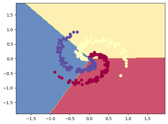
But, if you were to try to use a regular classification model to make predictions on this data, you would not get very great results. This data cannot be cleanly divided linearly, so a linear classifier simply cannot represent it as accurately as we would like. Here is what it looks like when a linear classification model tries to represent a dataset similar to ours:
Artificial Neural Networks
Artificial neural networks are one way to represent more complex data like we have in our data set. At their core, artificial neural networks are computerized abstractions which model the way we think the cells in the human brain make decisions in a simplified way. Or, they can be thought of as a group of many classification models arranged in layers, where the output from each layer is fed as input into the next layer. This allows the presence of specific features arising from relationships between the raw inputs to be fed to later classifiers, instead of just the raw data itself. This article assumes you have an understanding of how a single linear classification model works. If not, I suggest reading earlier entries in this series.
But, simply combining multiple linear classifiers isn’t enough. We need the power to represent non-linearly separable data in order to classify our spiraling points. That is why nonlinear activation functions are introduced into each neuron of a neural network. For each neuron, a regular inference step is run first (dot product of our weights with our input data, plus our bias). Then, the result of that inference step is entered into the neuron’s activation function, which is a function that introduces some kind of nonlinearity into the equation. Common nonlinearities include ReLU and Sigmoid.
ReLU

Sigmoid

Combining Nonlinearities
By using nonlinearities, we can use our weights and biases to manipulate the positions and slopes of the “bends” in our nonlinear activation functions. This, in effect, results in a piecewise application of multiple transformed nonlinear functions that is able to fit data that cannot be separated by a single line. Throughout training, we find the values for weights and biases for our network that can create classifiers like this:
Weights
Much like in previous classifiers, weights are used in neural networks to multiplicatively scale input attributes. Each neuron in a layer of our network needs a number of weights equal to the number of inputs it is receiving, plus on bias. So, if our input data has N features, and we have M neurons in the first layer of our network, the first layer will have a matrix of weights of size NxM.
Biases
Similarly, biases augment the input attributes additively. Each neuron in a given layer of our network needs just one bias, so in a layer with N neurons, that layer will have a 1D matrix of biases of size Nx1.
The Forward Pass
The forward pass of a neural network is the inference step, where we make predictions about data. It is where we use our weights and biases to compute the output for a layer of our network, then feed that output as input to the next layer. This process, carried out through the whole network, is known as the forward pass.
How it Works
Follow along with my explanation using this notebook.
As I mentioned, neural networks are essentially a number of classification models arranged into layers with outputs from one layer serving as inputs to the next. So, fundamentally, the forward pass of a neural network involves running an inference step using each layer of classifiers, in order, and feeding their results forward throughout the rest of the network. Let’s work through a small example, based on our spiral data set:
First, we need to get starting values for our weights and biases. We will need a matrix of weights for each layer of our network, and that matrix should be of size (i, n), where i is the number of inputs to a particular layer, and n is the number of neurons in that layer. This results in each of the n neurons having one weight per input it receives.. Then, we need our biases. As mentioned earlier, our biases will be a vector of size n, resulting in one bias per neuron. Weights values should start as small random values centered around zero, while bias defaults can all be zero.
So, for our example spiral dataset, let’s say we want a hidden layer with 6 neurons. Our weights matrix will then have a size of (2, 6) (2 features x 6 neurons), and the biases vector will have a size of (1, 6) (6 neurons).
weights = 0.01 * np.random.randn(2,6)
biases = np.zeros((1,6))
Now that we have our weights and biases, we need to run a basic inference step. We will take the dot product of x (our input data) with our weights. Because the size of x is (num_examples, 2), and the size of our first layer’s weights is (2, 6), the output of this operation will have a size of (num_examples, 6). Then, we just need to add our biases, and the first set of predictions is done.
output = np.dot(x, weights) + bNow, we need to pass the output through our activation function to get the final outputs for the layer. For this network, we will use the ReLU activation, so we will effectively floor each value in our output at zero.
output = np.maximum(0, output)And just like that, our forward pass through that layer is complete, and we have an output matrix of values which we will treat as our inferences for each example in the input for that layer. The output will be of size (num_examples, 6), and all the values will be floored at zero. Once we have that, we can continue with our forward pass, using the output from the previous layer as the input to the next layer, until we have run a forward pass through the whole network. The only step that might change in a network of fully connected layers is the activation function, which may be different from one layer to the next.
Particularly, the final layer of a neural network often uses a different activation function to generate useful results. In classifiers, one commonly used function is called the softmax function. It converts the outputs of the previous layers from more-or-less arbitrary numbers to a probability distribution of class labels. It works like this:
Each neuron in the output layer is mapped to a possible class label in the classification problem. So neuron 1 might correspond to the “red” group in our example above, neuron 2 to “blue, and neuron 3 to “yellow”. It is critical that the number of neurons in the final layer of the softmax activation function matches the number of class labels. Then, the softmax function:

is applied to convert the activations of each neuron to a probability. The sum of the outputs of each neuron in the layer will equal one, making the outputs a probability distribution. From there, extracting the predicted class is simple, as we just take the neuron corresponding to the label with the largest output, and that class is our model’s prediction. Intuitively, a high score relative to the other scores corresponds to a more sure prediction on our model’s part.
So, in our example above, let’s pass our output from the first layer to our output layer, which is using the softmax function:
exponentiated = np.exp(output)
softmax_output = exponentiated / np.sum(exponentiated , axis=1, keepdims=True)
So, we use first take e to the power of each value in our output, then, we divide each entry by the sum of all the entries to get a probability distribution. Now, all we have to do is find the index of the maximum value in softmax_ouput:
prediction = np.argmax(softmax_output, axis=1)And we have the class prediction of our model for each example in the data we passed to it. Not too complicated, right? Let’s take a look at how we might implement this in reusable, object-oriented code.
A Generic Implementation
We will implement our neural networks as modular classes that we can combine as we see fit. Full details for layers, activation functions, and how to use them can be found here and here.
Dense Layer
First, we will begin with the fully-connected, or dense, layer. A fully connected layer is a layer in a network where every input is mapped to every neuron with a unique weight for each connection. Our layer class will be in charge of taking the dot product of the inputs with weights, and then adding the biases:
class Layer_Dense:
  def __init__(self, n_inputs, n_neurons):
    '''initialize weights and biases'''
    self.weights = np.random.randn(n_inputs, n_neurons)
    self.biases = np.zeros(n_neurons)

  def forward(self, inputs):
    '''forward neural network pass, for inference'''
    self.inputs = inputs
    self.output = np.dot(inputs, self.weights) + self.biases

  def backward(self, dvalues):
    '''backward pass, to find gradient'''
    pass # coming soon...
As you can see, our Layer_Dense class contains three methods. The constructor simply initializes the weights and biases for the layer just like in our walkthrough. Note that weights has a entry for each combination of input and neuron in the layer (n_inputs x n_neurons), and there is one bias entry per neuron.
Meanwhile, the forward method implements the dot product of weights and inputs plus biases, just like in our walkthrough, and stores them in self.output. This allows us to modularly chain layers together. It also stores the inputs used to generate the outputs. The reason for this, as well as the backward method, will become apparent later, when we are learning about backpropagation. Stay tuned!
ReLU
We do the same with the ReLU implementation. The forward method floors all the values of the inputs at 0 to implement the activation function. The backward method will be shown later.
class Activation_ReLU:
  def forward(self, inputs):
    '''apply ReLU activation function to inputs'''
    self.inputs = inputs
    self.output = np.maximum(0, self.inputs)

  def backward(self, dvalues):
    '''backward pass, to find gradient'''
    pass # coming soon...
Softmax
Here is the class implementation for the softmax activation function. Just like the other two, we will show the backward implementation later in the post.
class Activation_Softmax:
  def forward(self, inputs):
    '''apply softmax activation function to inputs'''
    self.inputs = inputs
    exp_values = np.exp(inputs - np.max(inputs, axis=1, keepdims=True)) #get unnormalized exp values
    probabilites = exp_values / np.sum(exp_values, axis=1, keepdims=True)
    self.output = probabilites

  def backward(self, dvalues):
    '''backward pass, to find gradient'''
    pass # coming soon...
Class-Based Forward Pass
Now that we have reusable implementations, let’s take a look at what a forward pass, or inference step, might look like with our class implementations. Recall our dataset, which has this form:
| x | y | class (color) |
| 0 | -0.85 | 1 (blue) |
| 0.75 | 0.25 | 2 (purple) |
| … | … | … |
With that in mind, here is a forward pass using our classes:
X = our input data...

#create first layer and activation
dense1 = Layer_Dense(2, 3)    # 2 features x 3 neurons
activation1 = Activation_ReLU()

#create second layer and activation
dense2 = Layer_Dense(3, 3)    # 3 inputs x 3 neurons
activation2 = Activation_Softmax()

#input through first layer
dense1.forward(X)
activation1.forward(dense1.output)

#first layer output through second layer
dense2.forward(activation1.output)
activation2.forward(dense2.output)

#get prediction
prediction = np.argmax(activation2.output, axis=1)
The basic idea is that we take the input and pass it to a dense layer. Then, we take the output from that, and pass it to a ReLU activation function class. We then pass the output of the activation function to the next dense layer. This is repeated until we reach the last layer, where, instead of passing its output to a ReLU function, we pass it to a Softmax activation, which produces class probabilities.
Conclusion
So, we have a complete, generalized, class-based implementation of the forward pass of a neural network. This means that we can use our neural network to make predictions. But currently, we are using a model initialized with random weights and biases to make predictions, which means that its predictions are not very useful. We need to find a way to tune our weights to make them work better. And to do that, the first step is the implementation of the backward pass.
The Backward Pass
If the forward pass is the way to use a neural network to make a prediction, then the backward pass is the way to make the predictions generated by a neural network useful. You see, on a fundamental level, our network makes its predictions by applying weights and biases to the input. But, using random weights and biases like we have so far will result in, well, random predictions that do not tell us anything useful about the input data. This is where the backward pass comes in. By performing a backward pass on our network, we can find the values for weights and biases that make our network produce useful predictions.
Follow along in this notebook.
Getting Started: Finding the Gradient
In order to make our model produce useful predictions, we need an idea of what a “useful” prediction is. Obviously, in plain english, we can say, “a prediction is useful if the correct class is selected”. But, this definition leaves a lot of important details out. For one thing, recall how our softmax layer produces probabilities? Well, we want our classifier to produce high probabilities for the correct class, and low ones for the incorrect class. That means a prediction of 0.8 for correct and sum of 0.2 for all incorrect is much better than 0.51 for correct, and sum of 0.49 for incorrect. A binary correct/incorrect method for calculating usefulness does not quantify this.
Additionally, the english definition cannot be used by a computer program. We need to translate it into a mathematical function that describes the usefulness of the predictions generated by the model. This function might take the form of a function that accepts the final outputs of the last layer of the network as inputs, and produces high output when the predictions are very bad, and output approaching zero as the predictions become more and more useful. This is exactly what a loss function does.
Loss Function
A loss function is a mathematical function that uses a model’s predictions alongside the ground truth labels for the data to quantize our level of unhappiness with the predictions produced by the model. So, as mentioned before, a loss function should return a higher value when our model produces bad predictions, and it should produce low output when our model’s predictions are useful.
A loss function is applied to output from our network after a forward pass has been completed. The output should be taken from the network and passed through the loss function. Commonly, the average loss is then calculated from the loss produced per-sample, and this value is used to determine how happy we are with the model’s performance.
For this post, we are going to use a loss function called categorical cross-entropy. Categorical cross entropy is a loss function commonly paired with a softmax output layer that is used in classification problems where we have more than two classes. This function works by penalizing a high probability score for an incorrect label with a high output value and rewarding a high score for a correct value with low output. It can be defined mathematically like so:
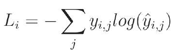
In this formula, i is the ith sample of the set, and j a variable used in the summation to iterate over each entry in each of y and y-hat. y, as you might expect, contains the ground truth, or target output for the classifier (what we want it to output), while y-hat contains what the network actually generated as output.
Here is an example of what the loss calculation for a sample where our class outputted the highest probability for the correct class. Note the relatively low loss output:
y_i =     [  0,   0,   1,   0 ]
y-hat_i = [0.1, 0.2, 0.6, 0.1 ]
j = 0 to 3


log_e(y_ij)   | y_i
______________|___
-2.30         * 0 = 0
-1.60         * 0 = 0
-0.51         * 1 = -0.51
-2.30         * 0 = 0
_____________________________
		   -0.51 * -1 = 0.51, Loss = 0.51
Now, let’s compare that to the exact same y-hat values, but now the correct class is at index 0 instead of 2:
y_i =     [  1   0   0   0 ]
y-hat_i = [0.1 0.2 0.6 0.1 ]
j = 0 to 3

log_e(y_ij)   | y_i
______________|___
-2.30         * 1 = -2.30 +
-1.60         * 0 = 0 +
-0.51         * 0 = 0 +
-2.30         * 0 = 0 +
_____________________________
		    -2.3 * -1 = 2.3, Loss = 2.3
When we assign a high probability to the incorrect class, our output is significantly higher… which is exactly what we want. By doing this, we are punishing high scores for incorrect values with a higher loss output, and rewarding high output on the correct class with low loss output. This allows us to quantify our unhappiness with our network’s output, which gives us a basis for discovering how to adjust our weights and biases to reduce this unhappiness.
Let’s take a quick look at an implementation for our loss function in python:
#loss functions
class Loss:
  def calculate(self, output, y):
    '''calculate the loss given model output and ground truth values'''
    sample_losses = self.forward(output, y)
    data_loss = np.mean(sample_losses)
    return data_loss


class Loss_CategoricalCrossEntropy(Loss):
  def forward(self, y_pred, y_true):
    '''forward pass through the cross entropy loss function'''
    #get number of samples in a batch
    samples = len(y_pred)

    #clip data to prevent divide by 0
    y_pred_clipped = np.clip(y_pred, 1e-7, 1 - 1e-7)

    #probabilities for target values
    if len(y_true.shape) == 1:
      correct_confidences = y_pred_clipped[range(samples), y_true]
    elif len(y_true.shape) == 2:
      correct_confidences = np.sum(y_pred_clipped*y_true, axis=1)

    #calculate loss
    negative_log_likelihoods = -np.log(correct_confidences)
    return negative_log_likelihoods

  def backward(self, dvalues, y_true):
    '''backward pass through the cross entropy loss function'''
    pass # coming soon...
The first thing you will notice is that we defined an interface, Loss. This reduces code duplication, as it allows us to get the average loss for a batch just by inheriting from it. In Loss_CategoricalCrossEntropy, we inherit from Loss and implement the math we just walked through in the forward method using numpy.
We take the values our model produced as its prediction, and, after ensuring we avoid divide-by-zero errors, pull out the score assigned to the correct label (we only take the correct one because the target value for incorrect labels is zero, meaning they would be zeroed out by the multiplication operation between y_ij and y-hat_ij in the formula). Then, we take the log base e of each prediction made for the correct value, and multiply it by -1. This gives us our cross-entropy loss for each sample. Then, we can the calculate method of the Loss superclass to get the average loss across all of the samples passed to the classifier.
Reducing Loss by Descending the Gradient
Now that we have a mathematical function that tells us numerically how good/bad our neural network’s classifications are, and an implementation of that function in python, we have a clear goal: we need to get the output of this function to be as low as possible. This will minimize our unhappiness with our output, and consequently cause our model to make more useful predictions.
To do this, we will descend the gradient using calculus. In calculus, we can take the derivative of a function with respect to some other variable to find it’s rate of change. By finding it’s rate of change with respect to some variable, we can determine which way we need to move the parameters we control to increase or decrease its output. Let’s take the function y = 2x as an example. The derivative of this function with respect to x is 2. 2 is also the slope of this function:
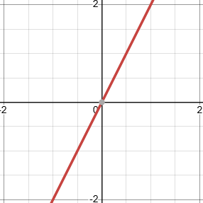
In this case, the derivative being equal to 2 tells us that for every increase in the value of x by 1,, the output of the function will increase by 2. And every decrease in x by one will reduce the output of the function by 2. A quick check tells us that this is true:
| x | y |
| 1 | 2 |
| 2 | 4 |
| 3 | 6 |
| … | … |
y = 2x is a simple function, but the exact same principle applies to all functions. Why does this matter? Well, going back to our loss function, if we can find its derivative with respect to the weights and biases of our network, then we can use that to determine what a change in a certain amount to one of the weights/biases will do to the output (the total loss). And, if we can do that, we can use that information to figure out how to adjust each of the weights and biases in our network to move us towards a network that produces minimal loss, and thus the most useful classifications. But to do that, we will need what comes next: the chain rule.
The Chain Rule
Now that we have seen how we can understand the relationship of each input to our loss function with the output value of that loss function using the derivative, we need a way to extend that principle all the way back to our weights and biases. If we can understand how much a change in a given weight value will increase or decrease our loss, we can determine how we should change each weight and bias in order to minimize the loss on our training data. To do that, we have to use the chain rule.
The chain rule is a fundamental idea in calculus that is used to calculate the derivative of a composite function, or a function inside of another function. At its core, an artificial neural network is just a bunch of mathematical functions nested together into one large function. Simply put, the chain rule states that the derivative of a composite function is equal to the derivative of the outer function evaluated at the inner function times the derivative of the inner function. It allows us to find the derivatives of complex functions by chaining together the derivatives of the simpler functions that make it up. The chain rule is written like this:

This means that by finding the derivative of smaller components of the full neural network function, such as the derivative of the just the loss function, the ReLU activation function, and other component functions, we can find the full derivative of the loss functions with respect to each weight and bias in the network. Once we have that, we can easily make changes to the weights and biases to reduce the loss on our training data. Let’s take a look at how we might go about implementing this on our network layers.
Implementing It
As we implement our backward pass (also known as backpropagation), or the process of using the chain rule to determine how to update each parameter of our neural network, to descend the gradient, we will need to revisit the implementation of the classes we began in the section on the forward pass. Remember the backward method stub that we put on the dense layer, activation, and loss functions? Well, we will be implementing those in a way that uses the chain rule to backpropagate through the network with the chain rule. Each of those methods took a single parameter, dvalues. We will use this value, which will be passed in by the next layer in the network (the operation the current one passes its outputs to in the forward pass), to compute the derivative of the current layer with respect to its inputs and, in the case of Layer_Dense, its weights and biases.
Chain Rule Implementation
So, without further ado, lets take a look at how to implement the chain rule to conduct a backward pass through our neural network. We will do this by implementing the backward stub on each of the classes we built out. For brevity, I will omit code we have already seen. Check here for full implementation details.
I implemented this class to combine the calculation of loss with the final softmax activation:
class Activation_Softmax_Loss_CategoricalCrossEntropy():

  def __init__(self):
    self.activation = Activation_Softmax()
    self.loss = Loss_CategoricalCrossEntropy()

  def forward(self, inputs, targets):
    '''
       forward pass of the softmax activation function
       and cross-entropy loss function
    '''
    self.activation.forward(inputs)
    self.output = self.activation.output
    return self.loss.calculate(self.output, targets)

  def backward(self, dvalues, y_true):
    '''
       backward pass of the softmax activation function
       and cross-entropy loss function
    '''
    samples = len(dvalues)
    # If labels are one-hot encoded,
    # turn them into discrete values
    if len (y_true.shape) == 2 :
      y_true = np.argmax(y_true, axis = 1 )
    # Copy so we can safely modify
    self.dinputs = dvalues.copy()
    # Calculate gradient
    self.dinputs[ range (samples), y_true] -= 1
    # Normalize gradient
    self.dinputs = self.dinputs / samples
As you can see, this class combines the calls to both forward and backward for the final activation and loss function into a single convenient operation. Because this is the output layer of the network, we pass the output of this layer (layer.output) into it’s own backward method as dvalues. The backward pass begins by converting one-hot encoded truth values to discrete values (index of the correct entry). Then, it computes the gradient with respect to the inputs and divides the gradient by the number of samples. The result tells us how a change in the inputs to this layer will affect the values outputs of the layer. We save this in dinputs.
Before the softmax activation in our network came a dense layer. So now, we need to use the chain rule to take another step back through the network towards our goal. We will feed the dinputs value we calculated in the output layer into the backward method of our Layer_Dense instance as the dvalues parameter. Let’s take a look at the implementation of that method now:
class Layer_Dense:
  ...
  def backward(self, dvalues):
    '''compute the gradient using the chain rule, and perform parameter updates'''
    self.dweights = np.dot(self.inputs.T, dvalues)
    #chain rule (partial derivative here * derivative from previous layer)
    self.dbiases = np.sum(dvalues, axis = 0 , keepdims = True)
    #chain rule again, partial derivative here is 1 so i don't write it
    self.dinputs = np.dot(dvalues, self.weights.T)
    #chain rule again (partial derivative here * derivative from previous layer)
Notice that the effect of this method is the same. We use dvalues, which was passed by the previous layer, to compute self.dweights, self.dbiases, and self.dinputs. The latter will be passed as dvalues to the backward method of the previous layer (the activation function of the previous dense layer). Meanwhile, the former will be used to inform the change to the weights and biases (the parameter update) of this layer (details coming later).
The activation function of all the layers in our network except the last one (which used softmax) is the ReLU function. Let’s take a look at the implementation of the backward pass through this function.
class Activation_ReLU:
  ...
  def backward(self, dvalues):
    '''compute the gradient for this activation function using the chain rule'''
    self.dinputs = np.zeros(self.inputs.shape)
    self.dinputs[self.inputs > 0] = 1
    self.dinputs *= dvalues
Once again, we take in dvalues, which we will use to fulfill the chain rule. The derivative of the max is 1 on the larger input, and 0 on the smaller. This checks out because changing the smaller of the two inputs will not have any impact on the output of the overall function. Unless, of course, that adjustment makes the smaller input larger than the one that was previously larger. On the larger output, meanwhile, the derivative is 1, because a change in the value of the larger input by x will result in a change in the output of the max function by x.
After getting the derivative of the max function, we just apply the chain rule by multiplying dinputs by dvalues, and save the result to pass to the previous layer. And we repeat that until we reach the beginning of the network, calling backward on each layer and passing in layer.dinputs into it as the dvalues parameter.
So, now we’ve got backward defined in each class. Let’s take a look at how a complete backward pass works under this network implementation.
#data
y = (the truth labels)

#create network
dense1 = Layer_Dense(2, 3)
activation1 = Activation_ReLU()
dense2 = Layer_Dense(3, 3)
activation2_and_loss = Activation_Softmax_Loss_CategoricalCrossEntropy()

#forward pass
...

#backward pass
activation2_and_loss.backward(activation2_and_loss.output, y)
dense2.backward(activation2_and_loss.dinputs)
activation1.backward(dense2.dinputs)
dense1.backward(activation1.dinputs)
Notice how dinputs, which is calculated in the backward method of each layer, is passed as dvalues into the backward method of the preceding layer. This is the core of the chain rule, which allows us to go backward from the derivative of the loss function, to the derivative with respect to the weights and biases of the network. This is bulk of our implementation of backpropagation, which we want to use to find weights and biases that cause our network to produce useful output. By doing this all the way through the network, we were able to find dweights and dbiases for each dense layer in out network. These will be used to calculate our parameter update.
Parameter Update Implementation
Once we have used the chain rule to find the derivative of the loss function of our network with respect to our weights and biases, we can predict how changing each weight and bias will affect the loss output of our network. We want to change our weights and biases so that our loss (unhappiness with the outputs of the network) is minimized. Conveniently, one of the things that derivatives tell us is the gradient of the function with respect to the inputs to the loss function. dinputs tells us something about the gradient of the loss function with respect to the inputs, and dweights (and dbiases) tells us about the gradient with respect to the weights of a particular layer. This means that it tells us which way we need to change inputs to the function to create an increase or a decrease in the function’s output.
Armed with this knowledge, we can make a small change to the weights and biases of each dense layer in our neural network based on the derivative of the function with respect to that weight or bias. This step is called our parameter update.
Remember how in the backward method of the dense layer class, we calculated both dinputs, dweights, and dbiases. Well, dinputs was used to complete a backward pass through the network via the chain rule, but dweights (and dbiases) is what we are really interested in. dweights (and dbiases) tells us about how a change in the value of a particular weight (or bias) will affect the output value of the loss function. Now, recall that weights and biases are currently randomly initialized, but we want them to be set such that we minimize the output of that function. Because we can change our weight and biases freely (unlike inputs, which come from X and are measured values), we are free to make a change informed by dweights and dbiases to minimize our loss, and thus make our network make useful predictions.
In practice, this means simply updating the weights and biases of the layer in the negative direction of the gradient. Recall that gradient can be compared with the slop of a line, and that slope = rise/run. If we have the function L = 2x, where w = slope, then dweights would be equal to 2. To reduce L, we would want to make w smaller, because the gradient tells us that as w decreases, L will also decrease. We do this by adjusting w in the opposite direction of its current value. Since it is positive, we move it in the negative direction by a certain amount.
How much do we adjust it by? Well, that is where the learning rate comes in. The learning rate, a small constant that controls how large our parameter updates are, should be multiplied by our gradient to get the parameter update. So in the case of L = 2x, where learning rate is 0.1, our parameter update could be calculated:
z = -1 * LR * w = -1 * 0.1* 2 = -0.2
Note the -1. That ensures we move in the opposite direction of the gradient, which ensures we move towards a minimum, not a maximum.
So now, add that to the current value of w, and the function becomes L = 1.8x. And for the same value of x, our new function returns a smaller loss value, which tells us that our parameter update did its job.
The principle is the same for updating the weights and biases of a dense layer of a neural network. Simply take dweights, and multiply it by the learning rate, and subtract that value from the current weight values of the layer. Likewise for biases: dbiases * learning_rate, then subtract that value to layer.biases.
In code, a parameter update will look something like this:
#layer is an instance of Layer_Dense
#that has undergone backpropagation
LEARNING_RATE = 0.1

...

#calculate param updates
weight_updates = -1 * LEARNING_RATE * layer.dweights
bias_updates = -1 * LEARNING_RATE * layer.dbiases

#apply param updates
layer.weights += weight_updates
layer.biases += np.ravel(bias_updates)
This is the basic process of using backpropagation to update the weights and biases of our network. But, there are some improvements that can be made to avoid issues like overfitting and getting stuck in local minima. To solve these, we will implement optimizers, specialized classes that help us reach new standards of performance in our neural networks.
Optimizing Things
Explore my process of using optimizers here.
Optimizers are used to compute parameter updates for our neural network, and apply techniques that help us arrive at a more useful finished model after we are done training.
There are a range of different optimizers that are used under different circumstances to, well, optimize the performance of neural networks. Each of them works slightly differently, but all serve the same fundamental goal of finding the set of weights and biases for each layer of our network that minimize loss, and thus make the network produce the most useful results.
Basic Gradient Descent
One simple optimizer that sees a lot of use across many applications is called the Stochastic Gradient Descent Optimizer. This optimizer works by computing the gradient with respect to a single sample from the training set, and then making the parameter update like we saw above based on the gradient from that one sample.
Building upon stochastic gradient descent (SGD) is batch gradient descent (BGD). This optimizer works identically to SGD, but instead of just one sample, it takes a batch of samples, computes the average gradient from all those samples, and computes that parameter update based on all those samples.
Learning Rate Decay
Learning rate decay is one way that we can improve the training process of our model using our optimizer. Learning rate decay is when we start the learning rate for our model at a relatively high learning rate, and gradually reduce it throughout training using a concept known as exponential decay.
Under exponential learning rate decay, we take two hyperparameters: a learning rate and a learning rate decay value. We use these values to calculate the learning rate using the following formula:
learning_rate = learning_rate * ( 1 / ( 1 + decay * iterations ) )Where iterations is equal to the number of times we have updated the parameters of the network. We then use this learning rate to compute the parameter update, and apply that scaled parameter update to the parameters.
Momentum
Another augmentation that is often added to optimizers like SGD is momentum. This essentially means that, in addition to updating in the direction of the gradient, a concept like inertia is added to the parameter update to allow the model to escape local minima in the loss function. To demonstrate how this helps, let’s take a look at this loss function:
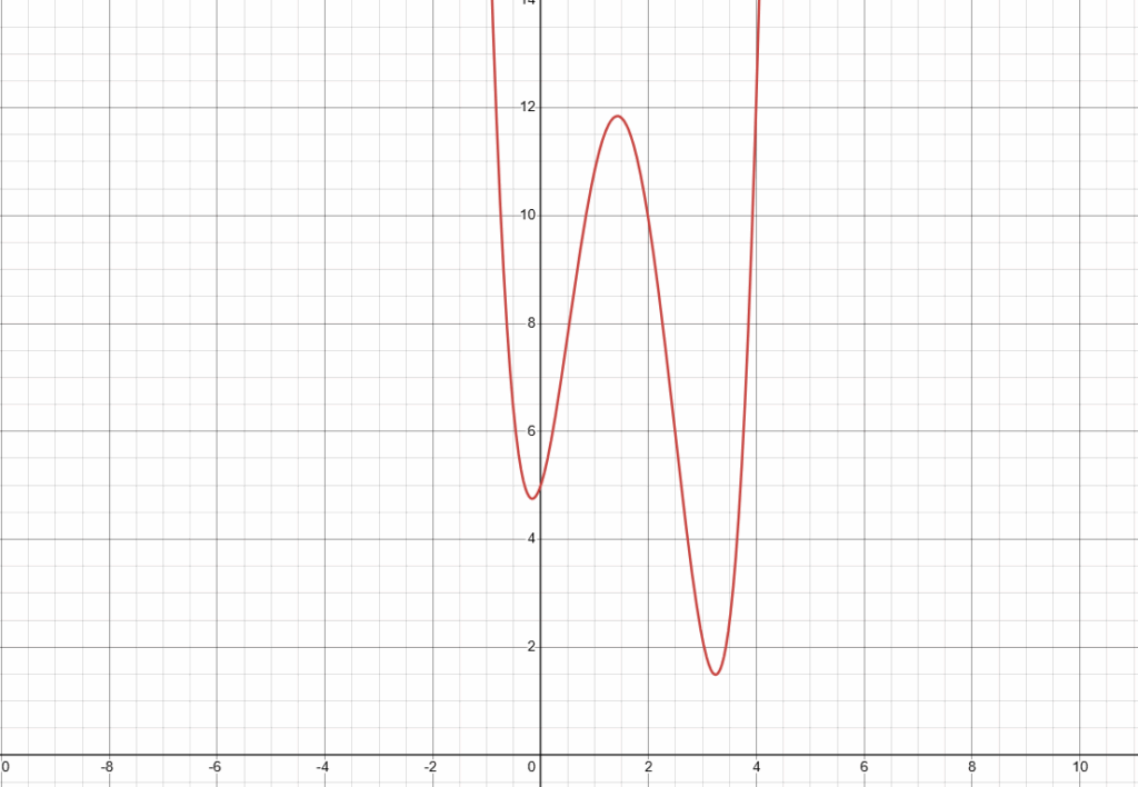
As you can see in this picture, we have a function with two local minima. As you can see, the rightmost minima is smaller than the leftmost, making it the most optimal value. Now, let us imagine we are descending the gradient from left to right. If we use a simple gradient descent, what will happen is either we will get stuck the leftmost minima because the learning rate is too small to overcome the peak between them, or the learning rate will be so large that training cannot proceed effectively. This means that we would never reach the optimum value (absolute minimum).
Momentum solves this by adding another factor to the next parameter update: the parameter update that preceded it. By taking into account the magnitude and direction of the previous parameter update, we can escape the local minima in many cases. Think of it this way: As we descend the gradient from the left, we pick up momentum. This momentum, like on a roller coaster, allows us to overcome the small peak between the minima. We then descend again down to the absolute minimum, and then spend the rest of our momentum swaying back and forth in the valley until we end up at the lowest point.
Below, we have an implementation of SGD with learning rate decay and momentum:
class Optimizer_SGD:
  def __init__(self, learning_rate = 1.0, decay=0.0, momentum=0.0):
    self.learning_rate = learning_rate
    self.current_learning_rate = learning_rate
    self.decay = decay
    self.iterations = 0
    self.momentum = momentum

  def update_params(self, layer):
    '''update the parameters of a layer using the SGD optimizer'''
    #im momentum is used
    if self.momentum:

      #create momentum arrays for a layer if they dont exist
      if not hasattr(layer, 'weight_momentums'):
        layer.weight_momentums = np.zeros_like(layer.weights)
        layer.bias_momentums = np.zeros_like(layer.biases)

      #build weight updates with momentum...
      #by taking previous updates times retaining factor, and
      #then updated with current updates
      weight_updates = self.momentum * layer.weight_momentums - self.current_learning_rate * layer.dweights
      layer.weight_momentums = weight_updates

      #build bias updates with momentum
      bias_updates = self.momentum * layer.bias_momentums - self.current_learning_rate * layer.dbiases
      layer.bias_momentums = bias_updates

    #otherwise, perform momentumless SGD
    else:
      weight_updates = -self.current_learning_rate * layer.dweights
      bias_updates = -self.current_learning_rate * layer.dbiases

    #parameter updates
    layer.weights += weight_updates
    layer.biases += np.ravel(bias_updates)

  def pre_update_params(self):
    '''implement learning rate decay'''
    if self.decay:
      self.current_learning_rate = self.learning_rate * (1 / (1 + self.decay*self.iterations))

  def post_update_params(self):
    '''increment the iteration count, for lr decay'''
    self.iterations += 1
We can then use the optimizer in a training loop like this:
#define network
...
optimizer = Optimizer_SGD((learning_rate = 1.0, decay=5e-7, momentum=0.1)

#train the model
for epoch in range(TRAIN_EPOCHS):

  #other training steps
  ...

  #update parameters
  optimizer.pre_update_params()
  optimizer.update_params(sgd_dense1)
  optimizer.update_params(sgd_dense2)
  optimizer.post_update_params()
Adam
The most popular optimizer today is the Adam Optimizer. Short for Adaptive Momentum, it combines the momentum concept from SGD with adaptive learning rates for each parameter (the main feature of RMSProp, another optimizer that, for brevity, is not discussed in full here) and a bias correction mechanism to result in a powerful optimizer. I will now briefly touch on the two concepts we have not already discussed: adaptive learning rates and bias correction.
Adaptive Learning Rates
This is the core of what RMSProp does. Basically, we keep a cache that stores a moving average of all parameter updates for each parameter. Then, when performing the parameter update, we divide by this cache. Because the average update for each parameter will be different based on the gradient of the function, this has the effect of creating a unique learning rate for each parameter, where the updates for parameters with a large cache entry will be smaller, and those for ones with a smaller cache entry will be larger. This results in a network using more of its parameters to learn the training set by making the updates for that parameter move more quickly towards their optimum values, and slows down ones that are used a lot to help negate overfitting.
In the Adam Optimizer, the cache for weights is calculated like this (biases are done similarly):
weight_cache = np.zeros_like(weights)
weight_cache = rho * weight_cache + (1 - self.rho) * dweights
Where rho is a hyperparameter, and weights are the weights of the current layer. weights are the weights of the layer, and dweights is the gradient with respect to the weights. Then, the parameter update is performed like so:
weights += -1 * ( ( lr * weight_momentums ) / ( np.sqrt(weight_cache) + epsilon ) )Where lr is the learning rate and weight_momentums are the momentums we discussed earlier in the section on momentum. If that doesn’t quite make sense, that’s ok, it will come together in the final implementation.
Bias Correction Mechanism
The Adam optimizer uses both adapative learning rates (bias_cache) and momentum (bias_momentums) to help find the correct bias values. Both of these matrices are initialized to zeros at all entries. To help them get to useful values more quickly in the training process, the Adam optimizer adds a bias correction mechanism. It works by increasing the magnitude of the momentum and cache for the biases, resulting in much faster training in the first iterations of training, and then gradually tapering off as more useful values for training are added to the momentum and caches.
Mathematically, we accomplish this by adding a divisor to the calculation of the bias_cache and bias_momentums. Using the function 1 - (beta_1 ** step), where step is the iteration of training we are on, and beta is a hyperparemeter that represents a fraction of the momentum to apply (beta_1 for bias_momentums, and beta_2 for bias_cache). So, on the first step, when beta_1 = 0.9
1 - (0.9 ** 1) = 1 - 0.9 = 0.1Meanwhile, as step gets very large,
1 - (0.9 ** ∞) ≈ 1 - 0 = 1So, as we can see, when step is small, we divide by a small fractional value, which results in the change to bias_momentums being scaled up drastically. Meanwhile, as step gets bigger, we divide by a number closer and close to 1, which means that we return to a regular-sized change to the momentums. And the change to bias_cache is calculated identically, except using beta_2 instead of beta_1. We can see this in action in the optimizer code:
bias_momentums_corrected = bias_momentums / (1 - beta_1 ** (step + 1))A similar calculation is used to correct the bias_cache. Now, let’s take a look at the full Adam optimizer in code:
Code Implementation
Here is the full implementation of the Adam optimizer:
class Optimizer_Adam:
  def __init__(self, learning_rate = 1.0, decay=0.0, epsilon=1e-7, beta_1=0.9, beta_2=0.999):
    self.learning_rate = learning_rate
    self.current_learning_rate = learning_rate
    self.decay = decay
    self.iterations = 0
    self.epsilon = epsilon
    self.beta_1 = beta_1
    self.beta_2 = beta_2

  def pre_update_params(self):
    '''before the parameter update, perform learning rate decay'''
    if self.decay:
      self.current_learning_rate = self.learning_rate * (1 / (1 + self.decay*self.iterations))

  def update_params(self, layer):
    '''update the parameters of a layer using the Adam optimizer'''
    #create momentum arrays for a layer if they dont exist
    if not hasattr(layer, 'weight_momentums'):
      layer.weight_momentums = np.zeros_like(layer.weights)
      layer.weight_cache = np.zeros_like(layer.weights)
      layer.bias_momentums = np.zeros_like(layer.biases)
      layer.bias_cache = np.zeros_like(layer.biases)

    #update momentum with curretn gradients
    layer.weight_momentums = self.beta_1 * layer.weight_momentums \
                            + \
                            (1 - self.beta_1) * layer.dweights
    layer.bias_momentums = self.beta_1 * layer.bias_momentums \
                           + \
                           (1 - self.beta_1) * layer.dbiases

    #get the bias-corrected corrected momentum
    #this speeds up training when self.iterations is low allowing
    #for tables to escape their zero-initialization more easily
    weight_momentums_corrected = layer.weight_momentums / (1 - self.beta_1 ** (self.iterations + 1))
    bias_momentums_corrected = layer.bias_momentums / (1 - self.beta_1 ** (self.iterations + 1))

    #update the weight cache with the squared values of current gradients
    layer.weight_cache = self.beta_2 * layer.weight_cache + (1 - self.beta_2) * layer.dweights ** 2
    layer.bias_cache = self.beta_2 * layer.bias_cache + (1 - self.beta_2) * layer.dbiases ** 2

    #get the bias-corrected cached weights
    weight_cache_corrected = layer.weight_cache / (1 - self.beta_2 ** (self.iterations + 1))
    bias_cache_corrected = layer.bias_cache / (1 - self.beta_2 ** (self.iterations + 1))

    #perform parameter updates
    layer.weights += -self.current_learning_rate * \
                      weight_momentums_corrected / \
                      (np.sqrt(weight_cache_corrected) + self.epsilon)
    layer.biases += np.ravel(
                      -self.current_learning_rate * \
                      bias_momentums_corrected / \
                      (np.sqrt(bias_cache_corrected) + self.epsilon)
    )

  def post_update_params(self):
    '''increment the iteration count, for lr decay'''
    self.iterations += 1
Training Results
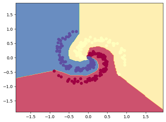
Now, at long last, we can get back to the results on the spiral dataset. I trained two identical models, one with an SGD optimizer, and one with an Adam optimizer. View this notebook to see the detailed network architectures and how I actually used the classes given here to train the models.
Here are the classifiers on the spiral dataset that each of my models produced. SGD-trained is on the left, and Adam-trained on the right. They both resulted in very high levels of accuracy on the test set
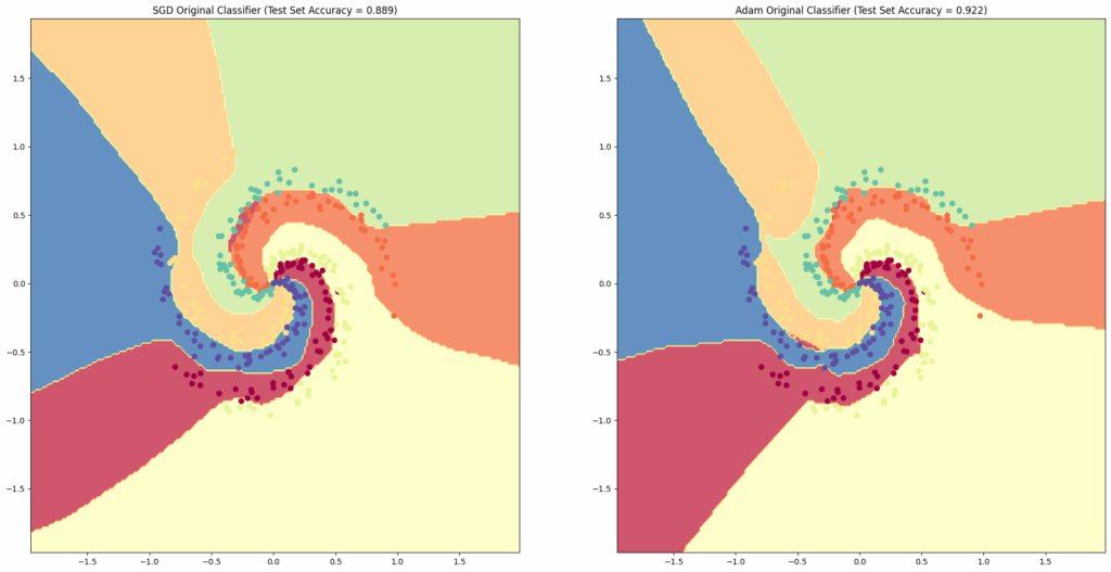
As you can see, by using artificial neural networks to classify this complex, non-linearly separable dataset, we are able to create a classifier that generalizes to the trends implicit in the data very well. And, thanks to the easy-to-use, object-oriented system we used to build our implementations, we can easily adapt our code to other datasets.
Conclusion
Artificial neural networks provide a powerful framework for building and training models to classify complex sets of non-linearly separable data. Implementing them from scratch provided us with many insights into how they work behind the scenes, including the fundamental mathematical operations and principals that make them work. The framework we built here can be adapted to a diverse set of inference tasks, allowing us to apply the same methodology to many different problems.
Examples and full source code behind the examples found in this post can be found by viewing these three publicly-accessible colab notebooks:
I hope this guide has proven useful to you. Just writing it has been incredibly helpful in enhancing my understanding of neural networks. Please, feel free to reach out with any questions or advice you may have! Learning neural networks is both a fascinating journey and a useful skill! Thanks, and happy coding!
Leave a Reply