
How I Built a Powerful Binary Classifier From Scratch in Python

Hello, I hope you are doing well. This is the first entry in what I hope to make a series of articles documenting my journey into learning about the fundamentals of machine learning and AI by building the systems from scratch. This time, I will demonstrate how I built a powerful binary classifier from scratch in python using logistic regression. You can view the full Colab notebook I used in my project by clicking here, and use it to follow along. Let’s get started!
Online Shopping Dataset
To begin, we should get acquainted with our dataset. The professor who taught my introduction to machine learning class in school always said that machine learning is something like 90% data exploration and 10% model building and training. The point was, you need to be very familiar with the format and major features of your data.
So, with that in mind, let’s take a look at our dataset. For this project, I used the “Predict Customer Purchase Behavior Dataset” available from kaggle. It contains 1500 records about users of online shopping services, including their age, annual income, time spent on website, and more, and includes a label indicating whether they ended up making a purchase.
Here is a list of the features of our dataset:
- Age: customer’s age.
- Gender: 0 = male, 1 = female.
- Annual income: annual income of customer, in dollars.
- Number of purchases: number of other purchases made by the customer.
- Product category: 0 = electronics, 1 = clothing, 2 = home goods, 3 = beauty, 4 = sports.
- Time spent on website: time in minutes customer was on website.
- Loyalty program: 0 = not a member, 1 = member.
- Discounts available: number of discounts available, 0-5.
- Purchase status: this is the value we are trying to predict, whether the customer will make a new purchase or not, 0 = no purchase, 1 = purchase.
Here are a few example records from the dataset:
| Age | Gender | AnnualIncome | NumberOfPurchases | ProductCategory | TimeSpentOnWebsite | LoyaltyProgram | DiscountsAvailed | PurchaseStatus |
| 40 | 1 | 66120.26793867795 | 8 | 0 | 30.56860115599193 | 0 | 5 | 0 |
| 20 | 1 | 66120.26793867795 | 4 | 2 | 38.240096605544196 | 1 | 0 | 1 |
I loaded the csv data into a pandas dataframe, and did some basic data exploration on it to find the average, standard deviation, and other basic statistical variables for each feature. At this point, I wanted to see what my performance would be like without using any synthetic features or any other fancy tricks, so I decided to move on to preparing for the inference task.
Preparing the Data
After understanding my dataset and getting it loaded into my notebook, I had to get it ready to be used in my binary classifier. I started by dividing the data into training and test sets. The training set will be used to find good values for the weights and bias used in my logistic regression classifier (more on this later), and the test set will be used to evaluate how well those weights generalize to unseen data.
If you have any familiarity with machine learning whatsoever, you have likely heard of the concept of overfitting – when you create a set of weights that work well on your training data, but don’t do well on data the classifier has not seen before. This is because the weights are attuned to specific peculiarities of the training set that are not present in the wider world of examples. This is why we separate into training and testing sets, so that we can ensure we have not overfit our model to our training data by ensuring it performs well on our testing data.
X_train = data.iloc[:round(data.shape[0]*0.8)].drop('PurchaseStatus', axis=1)
X_test =  data.iloc[round(data.shape[0]*0.8):].drop('PurchaseStatus', axis=1)
y_train = data.iloc[:round(data.shape[0]*0.8)]['PurchaseStatus']
y_test = data.iloc[round(data.shape[0]*0.8):]['PurchaseStatus']
Now, X_train contains 80% of our dataset, not including the purchase status, X_test contains the other 20%, again, not including the label (purchase status). Meanwhile, y_train and y_test contain the labels for each example in X_train and X_test, respectively.
Now, I normalize the data by subtracting the mean and dividing by the standard deviation. Note that I only use the training set to compute the mean and standard deviation.
columns_to_normalize = ['Age', 'AnnualIncome', 'NumberOfPurchases', 'ProductCategory', 'TimeSpentOnWebsite', 'DiscountsAvailed']

# Normalize each column
for column in columns_to_normalize:
    X_train[column] = (X_train[column] - X_train[column].mean()) / X_train[column].std()
    X_test[column] = (X_test[column] - X_train[column].mean()) / X_train[column].std()
This squishes very large values down, making them play nice with python and producing more even weights as I move forward. Then, I decided to use an 80-20 split for my testing set to training set ratio. So, I train on 80% of the records, and test on the remaining 20%. I also had to divide the label (whether the customer made a purchase) from the other features of each example. Luckily, pandas made this simple:
Now, our data processing step is done, and we can move on to the exciting part: the inference task.
The Math Behind the Magic
You may recall that I mentioned that I would be using a logistic regression to make my classifications. “Logistic Regression” is just a fancy term for a mathematical function with two parts: a “predictor” (my term) part that applies learned weights and bias to input variables, and the sigmoid function, which maps the value from the former part to a value between 0 and 1. You can think of it like this: the “predictor” predicts whether the customer will make a purchase based on everything we know about them, and the sigmoid portion translates that prediction (some number) into a value that means something to us: a probability, or value between 0 and 1. With that said, here is the full mathematical function for logistic regression:
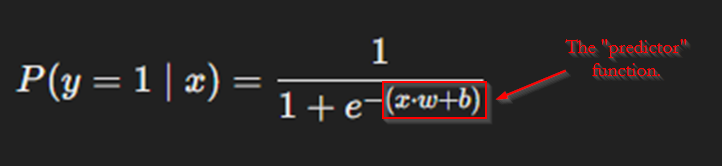
“Predictor” Function
Let’s look at the predictor function first. We will analyze how it works first, and then, we will translate it into python code. As noted above, this function is quite simple: it gives takes the dot product of a set of weights with a given example, and then adds a bias vector. Perhaps a concrete example will help.
| Age | Gender | AnnualIncome | NumberOfPurchases | ProductCategory | TimeSpentOnWebsite | LoyaltyProgram | DiscountsAvailed |
| -0.276668 | 1 | -0.481774 | -0.411048 | -1.409425 | 0.005862 | 0 | 1.433694 |
As you can see, we have an example here. This example has all its non-binary properties normalized. Let this example be “X”. That is part one of the predictor equation. Now, we need weights (w) and a bias (b). But, what do these mean?
Consider the line equation, y=mx+b. m controls how much the value of x influences the value of y due to their multiplicative relationship, while b defines a starting point for the relationship between the two, due to the additive relationship.
Consider, then, that the line equation is simply a simpler case of what we need here. We have a set of values X = [-0.276668, 1, -0.481774, -0.411048, -1.409425, 0.005862, 0, 1.433694]. So, we need a set of constants to multiply these to determine how much of an impact each of these attributes has on the label (y). We simply store each of these constants in the list of weights (w). And, we need a starting point, or bias (b), for the relationship. So, our more advanced case becomes:
y = x[0]*w[0] + x[1]*w[1] + ... + x[7]*w[7] + bBut what do we set the values of w and b equal to? We don’t know yet! So, begin by randomly setting them. We will explore how to set these values well later in the post.
It turns out, we can simplify this equation by using the dot product of x and w. The dot product does exactly what is listed in the equation above: it multiplies the values in x and w elementwise, and then adds the results together. So, the above equation becomes:
y = (x ⋅ w) + bNotice that this is where the labeled portion of the equation in the image above comes from. This can be easily translated into python, like this:
prediction = np.dot(X, weights) + bias
# weights = w, bias = b
So, going back to the example provided in the table above, let’s compute the answer. For simplicity, lets set w = [1, 1, 1, 1, 1, 1, 1, 1] and b = -10. Our predictor function, then would output:
y = (x ⋅ w) + b = (-0.276668 * 1) + (1 * 1) + (-0.481774 * 1) + (-0.411048 * 1) + (-1.409425 * 1) + (0.005862 * 1) + (0 * 1) + (1.433694 * 1) + (-10) = -10.139539
And just like that, we’ve got our prediction! -10.139539! But, what does that mean? Who knows! It is hard to make use of this number because we have no frame of reference for what that means. That is where the other portion of the equation comes in: the sigmoid function.
Sigmoid Function
Now, we have the ability to make a prediction. But, we need to translate the prediction – a seemingly arbitrary number, into something meaningful. Back in our original equation, we were calculating the probability of y given X… the probability of a customer making a purchase given all the information we know about them. The sigmoid function converts the result from our predictor function into a probability value between 0 and 1. Let’s take a look.
Here is a basic representation of the sigmoid function:
y = 1 / (1 + e^-x)Where e is the Euler’s number, and x is a given number… we will, of course, place the result of our predictor function there. But, how does this function work? Look closely at the denominator. Because e is positive, e^-x will always return a number greater than 0 (it may be very small, but it will never be 0 or less). Then, we add 1 to it. This is significant because it ensures that the denominator will always be larger than the numerator (which is 1). If you prefer it in mathematic terms, here it is:
For all n > 0,
                1 + n > 1
by the definition of addition of positive numbers?
This, in turn, matters because the overall fraction of 1 / (1 + e^-x) can never reach 1 with such a denominator, and it can obviously never reach 0 because of the 1 in the numerator. So, the sigmoid function provides a mapping of our predictor value to somewhere on the interval (0, 1). And, it just so happens that we can use values on this exact interval to represent probabilities. But more on this in a second. Now, let’s continue our example from before:
y = (x ⋅ w) + b = -10.139539 -> 1 / (1 + e^-(-10.139539))
  = 1 / (1 + 25,324.7890....) = 0.00003948...
This can be written in python like this:
prediction = np.dot(X, weights) + bias
mapped_prediction = 1 / (1 + np.exp(-prediction))
So, our prediction, after being mapped to it’s probability value, is 0.00003948…. Our classifier seems VERY sure that this customer will not make a purchase. But, in this case, it was dead wrong! This customer did make a purchase. So, what went wrong?
A Problem with Our Predictor
Well, do you remember when I said that we will initialize the weights and biases to random values? Well, it turns out that this doesn’t work too well. The weights and bias may not at all correspond to the actual relationship between the features and the label. In other words, the weight of “1” that we chose for the “AnnualIncome” feature, for example, may not be properly representing the relationship between how much the customer makes in a year and whether they will make a purchase on our site.
To solve this problem, we need a better way to choose our weights than randomly assigning them. But this will be addressed later. First, let’s translate all this math into good old-fashioned python code!
Writing the Classifier
Let’s take a look at the implementation of a binary classifier I built in python:
#create a logistic regression model that trains on accuracy using random small adjustments.
class LogReg:
  def __init__(self):
    '''initialize weights'''
    self.weights = np.random.randn(X_train.shape[1]) * 0.1  #want small weights, so multiply by 0.1
    self.bias = 0
    self.epoch_values = []
    self.training_progress = []

  def predict(self, X):
    '''predict the class of some samples (where x is a pandas dataframe)'''
    predictions = []
    for _, row in X.iterrows():
        xw = np.dot(row.values, self.weights) + self.bias
        sigmoid = 1 / (1 + np.exp(-xw))
        predictions.append(sigmoid)
    return predictions

  def fit(self, X, y, epochs=1000, lr=0.01, verbose=True):
    '''fit the model to the data, by using random small adjustments to the weights and bias'''
    #we will come back to this
    pass
So, we have a class with two methods: predict and fit. The constructor is fairly straightforward: we randomly create a weight for each feature in a record from our data, and we initialize our bias to zero. I also created a few lists to store data about our progress as we train the model, which is useful for seeing how our the weights and bias change in our model during the training process.
predict does just what we discussed above in all that math: for each example we pass into it using a pandas dataframe, it takes the dot product of the example with the weights array, and adds the bias (predictor function). Then, it uses the result (a single number) in the sigmoid function to translate our prediction into a probability of whether the customer made a purchase or not.
The fit method, meanwhile, is not defined above. The purpose of fit is to find a good set of weights and bias, so that our classifier can make predictions with a high level of accuracy.
Training the Model
There are some fairly advanced mathematical methods we could use to train this binary classifier, but I have not progressed to learning those yet (though I plan to soon!). So, I chose to use a relatively simple but quite effective method for this data set.
The method I chose involves keeping track of the set of weights and bias that produce the best accuracy, or proportion of correct labels to total records, on the training set. We start with the random weights and bias from our constructor, and iterate a set number of times (we decide this number), and make random, small adjustments to each weight and the bias (again, we decide the size of these adjustments). All the while, we make use of the training set to compare the accuracy of the updated weights with the accuracy produced by the best weights and bias we have found so far. If the new weights are better, we throw out the old best and keep the ones we just discovered. Otherwise, we throw out our new values and return to the old best values.
You may note that there are two values we get to decide: number of iterations and size of adjustments. These hyperparameters of our learning function are epochs and learning rate. They will be passed in to our fit function, so they can be adjusted.
#create a logistic regression model that trains on accuracy using random small adjustments.
class LogReg:
  ...
  def fit(self, X, y, epochs=1000, lr=0.01, verbose=True):
    '''fit the model to the data, by using random small adjustments to the weights and bias'''

    #saves for best weights and biases
    best_weights = self.weights
    best_bias = self.bias
    best_accuracy = 0

    #fit over the number of epochs
    for epoch in range(epochs):

      #determine accuracy of current weights and biases
      predictions = self.predict(X)
      for i in range(len(predictions)):
        if predictions[i] > 0.5:
          predictions[i] = 1
        else:
          predictions[i] = 0
      accuracy = np.sum(predictions == y)/len(y)

      #add current epoch to self.epoch_values
      self.epoch_values.append({
          'epoch': epoch,
          'accuracy': accuracy,
          'weights': self.weights.copy(),
          #call copy() because we want to pass by value, not by reference!
          'bias': self.bias
      })

      #save the weights and biases if they are better
      if accuracy > best_accuracy:
        if verbose:
          print(f"Epoch {epoch} found better accuracy: Accuracy = {accuracy}.  Updating weights and biases!")
        best_weights = self.weights.copy()  #call copy() because we want to pass by value, not by reference!
        best_bias = self.bias
        best_accuracy = accuracy
      else:
        self.weights = best_weights.copy()  #call copy() because we want to pass by value, not by reference!
        self.bias = best_bias

      #add current epoch's best values to self.training_progress
      self.training_progress.append({
          'epoch': epoch,
          'accuracy': best_accuracy,
          'weights': best_weights.copy(), #call copy() because we want to pass by value, not by reference!
          'bias': best_bias
      })

      #adjust weights and bias
      self.weights += lr * np.random.randn(X.shape[1]) #adjust weights randomly
      self.bias += lr * np.random.randn() #adjust bias randomly

    #use the best weights and biases (denoted by highest accuracy)
    self.weights = best_weights
    self.bias = best_bias
    if verbose:
      print(f"Done fitting!  weights = {self.weights}, bias = {self.bias}")
There is the implementation of the fit method. It works just like I described above. It iterates the designated number of times, generating new, slightly different weights from the current best, keeping the one that produces the better accuracy of the two on the training set. It also saves every set of weights it generates to the epoch_values list, and the best so far to the training_progress list. This is solely for record keeping and data visualization, as we will see. We are only concerned with finding the best values.
I should note, there are some issues with this training method. Chief among them is the fact that it has the potential to reach a set of weights that are good enough that no small adjustment within the learning rate can improve the performance, but that is not in fact optimal. As I continue my journey, I plan to explore better training methods that can do a better job of avoiding this problem.
However, on this particular data set, this method achieves quite good performance. It routinely trains to around 80% accuracy on the test set. However, accuracy on the training set doesn’t necessarily mean anything. I still need to evaluate on the test set to determine how well the model generalizes to new data.
Performance and Graphs
I tested the performance of the model using this code:
raw_predictions = lr.predict(X_test)
predictions = [
    1 if raw_predictions[i] > 0.5 else 0 for i in range(len(raw_predictions))
]
accuracy = np.sum(predictions == y_test)/len(y_test)
accuracy
It just runs predict on the test set, and calculates the accuracy. This model usually comes out to around 80% accuracy on the test set, which is very similar to the training accuracy levels. This tells us that the model generalizes well to data that it has never seen before, so it is a useful model!
There is one more little added feature of my implementation that provides interesting insights into how the model works under the hood. Remember those two lists, epoch_value and training_progress? Those contain all the data we generated throughout the training progress. It turns out, we can graph all those values out to see the relationship between each weight and the overall accuracy of the model during training. Using this code:
training_progress_epochs = [entry['epoch'] for entry in lr.training_progress]
training_progress_accuracies = [entry['accuracy'] for entry in lr.training_progress]

epoch_values_epochs = [entry['epoch'] for entry in lr.epoch_values]
epoch_values_accuracies = [entry['accuracy'] for entry in lr.epoch_values]
epoch_biases = [entry['bias'] for entry in lr.epoch_values]
epoch_weights = [entry['weights'] for entry in lr.epoch_values]

plt.plot(training_progress_epochs, training_progress_accuracies, label='training progress (accuracy)')
plt.plot(epoch_values_epochs, epoch_values_accuracies, label='epoch values (accuracy)')
plt.plot(epoch_values_epochs, epoch_biases, label='bias')

feature_labels = ["Age", "Gender", "Annual Income", "Number Of Purchases", "Product Category", "Time Spent On Website", "Loyalty Program", "Discounts Available"]
for i in range(len(feature_labels)):
  label = feature_labels[i] + " weight"
  weights = [epoch_weights[j][i] for j in range(len(epoch_weights))]
  plt.plot(epoch_values_epochs, weights, label=label)

plt.legend(bbox_to_anchor=(1, 1), loc='upper left')
plt.xlabel('epoch')
plt.ylabel('accuracy or weight/bias value')
plt.show()
I produced this graph when I trained a model on the testing set we built with learning_rate = 0.01 and epochs = 1000:
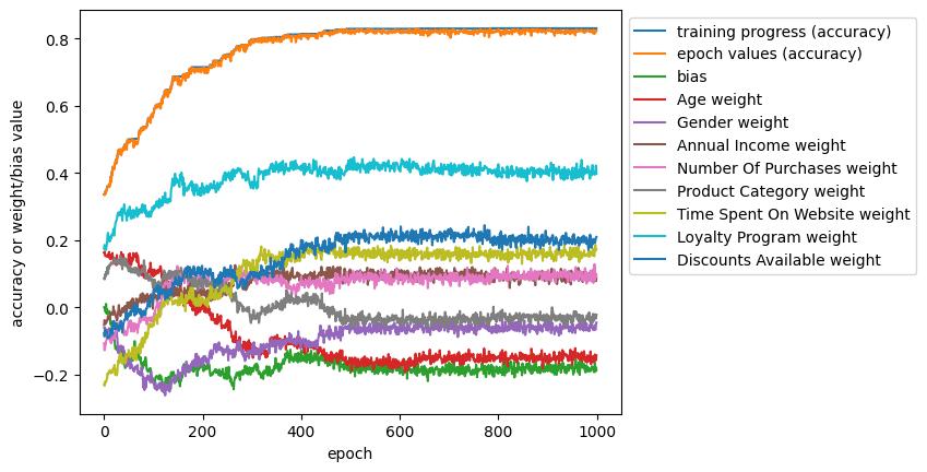
The training progress (accuracy) line represents the best accuracy we have achieved so far. Meanwhile, the epoch value (accuracy) represents the accuracy achieved by the new weights in this epoch. The training progress line acts as a ceiling for the epoch value line because it represents the best epoch value we have seen to that point. Meanwhile, the other lines are the weights and biases we are trying on this iteration. The small bumps in the lines are the random adjustments we make, while the overall trends appear when the small changes we make result in a new best accuracy (and so keep the updated value and make adjustments from that point instead of the old value of that weight or bias.
Briefly, I want to touch on how adjustments to the hyperparameters, learning rate and epochs would affect the appearance of this graph. A high learning rate would stretch out the x-axis, resulting in more iterations to find the best values. However, it appears from our graph to be unnecessary, as there was little improvement after epoch 500. Meanwhile, a higher learning rate would result in the line for all the weights and biases to be a lot more jagged as they are adjusted by larger amounts. A high learning rate might help us escape a set of decent but not optimal weights, but it could also struggle to zero in on a good set of weights. It is somewhat difficult to say whether this value should be changed, and in fact it is usually set empirically. But, we achieved good performance on this dataset, so it seems our value we chose worked well.
Conclusion
Binary classification is an important concept in machine learning, as it applies to a vast array of real-world issues. It is also a wonderful gateway into the world of machine learning and artificial intelligence, allowing beginners to wrap their heads around core concepts without overloading them with confusing concepts. It is easy to see the power of this concept: just by processing data, intelligently generating numbers, and using those numbers cleverly, we can predict whether a customer will make a purchase from our online store with ~80% certainty. That is pretty amazing!
I hope seeing how I built a powerful binary classifier from scratch in python has expanded your understanding of the process of classification tasks. All the code in this post was run in the context of a Jupyter notebook. Mine is hosted on Colab. Get access to it and run the code by clicking here. Understanding core concepts is crucial in this field, so be sure to take your time and really learn how everything works! Thank you very much for reading!
Leave a Reply